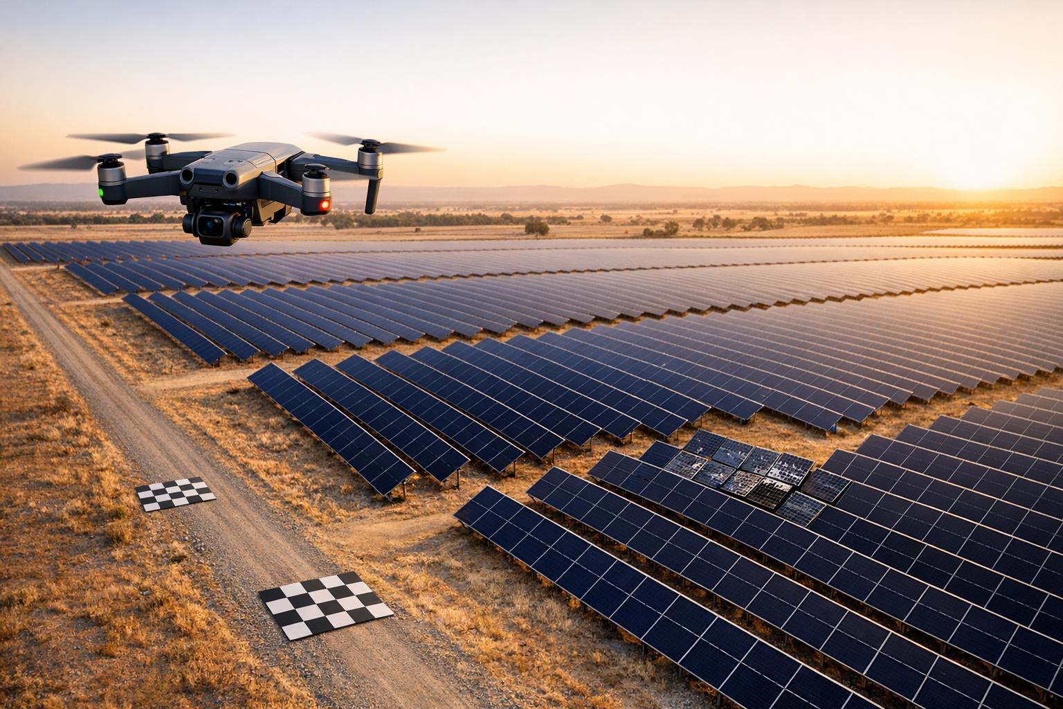
Drone photogrammetry is reshaping how we collect data for detecting anomalies. By capturing high-resolution images from drones flying at 100–200 feet, you can create detailed 2D maps and 3D models with sub-inch accuracy. This method is faster, safer, and less expensive than traditional surveys, cutting costs by up to 80% and speeding up workflows by 40%. Industries like construction, oil and gas, and agriculture are using these datasets to spot issues like structural misalignments, leaks, or crop stress.
By combining precise drone imagery with tools like RTK and PPK positioning, you can generate datasets ready for AI training in days. These datasets achieve pixel-level accuracy, enabling AI models to identify anomalies with 85–95% accuracy. Planning missions carefully - setting flight paths, ensuring image overlap, and using advanced software - ensures reliable data for labeling and analysis. Platforms like Anvil Labs streamline data management and annotation, helping teams integrate photogrammetry outputs into AI workflows efficiently.
For those starting out, focus on planning 5–10 drone missions to build a high-quality dataset. Use tools like Pix4Dmapper or Agisoft Metashape for processing, and annotate anomalies with software like CVAT or Labelbox. With proper planning and validation, drone photogrammetry can help you create reliable datasets for automated anomaly detection.

Drone Photogrammetry Workflow for AI Anomaly Detection Datasets
10 Tips for Drone Photogrammetry, by Hammer Missions

sbb-itb-ac6e058
Planning Drone Missions for Data Collection
Careful planning of drone missions is crucial for collecting high-quality data. Every detail - like altitude or image overlap - affects the accuracy of your dataset. Proper preparation helps avoid issues like coverage gaps, uneven image resolution, or inefficient use of flight time.
Setting Flight Boundaries and Altitude
Defining clear flight boundaries is key to both safety and effective data collection. Keeping the drone at a steady altitude ensures consistent image resolution and coverage. For systematic data capture, establish a "desired takeoff altitude" as the starting point for your mission.
Be mindful of obstacles that could interfere with the drone's path or signal. Strong winds can destabilize the drone and introduce data inconsistencies. In areas prone to signal interference - especially during beyond visual line of sight (BVLOS) operations - setting conservative flight boundaries helps maintain reliable communication. Industrial operations, for instance, consider signal delays over 2 seconds as anomalies.
Once flight boundaries are set, focus on optimizing image overlap and flight patterns to further improve outcomes.
Configuring Image Overlap and Flight Patterns
High image overlap is critical for photogrammetry software to accurately reconstruct 3D models and create seamless orthomosaics. Capturing multiple perspectives also helps in identifying subtle anomalies. Choose flight patterns based on the site’s layout: grid patterns are ideal for rectangular areas, while terrain-adaptive modes are better suited for regions with uneven elevation to maintain consistent image quality.
Using RTK/PPK for Accurate Positioning
RTK (Real-Time Kinematic) and PPK (Post-Processing Kinematic) systems significantly improve positional accuracy by correcting GPS errors using ground-based reference data. This level of precision - down to the centimeter - is vital for aligning 3D models and orthomosaics with real-world coordinates, especially when monitoring site changes over time. RTK provides real-time corrections, while PPK refines data post-flight. Together, these systems can enhance detection rates for anomalies, such as sensor faults, to over 99%. Incorporating RTK/PPK data ensures a dependable foundation for anomaly detection and site analysis.
Processing Photogrammetry Data
Once the mission planning is complete, the next step is processing the collected images to produce datasets that can be used for detecting anomalies. This involves converting raw drone images into orthomosaics and 3D models.
Creating Orthomosaics and 3D Models
Photogrammetry software uses feature detection algorithms (like SIFT or AKAZE) to match points across multiple images. The process unfolds in four main steps:
- Image alignment: Creates a sparse point cloud by matching features between overlapping images.
- Dense point cloud generation: Uses multi-view stereo matching to add more detail.
- Mesh creation and texturing: Produces 3D models with realistic textures.
- Orthomosaic generation: Projects the textured mesh onto a georeferenced flat surface to create a detailed map.
For anomaly detection, aim for a Ground Sample Distance (GSD) between 1–5 cm per pixel. For example, processing 500 images captured by a DJI Mavic 3 Enterprise at 400 feet (roughly 120 meters) can generate a 2 cm GSD orthomosaic covering 50 acres. On a mid-range GPU workstation, this takes about 2–4 hours.
Different software options cater to varying needs:
- Pix4Dmapper: Known for its integrated RTK support, it handles large datasets efficiently.
- Agisoft Metashape: Offers extensive customization through its scripting API, ideal for batch processing large datasets.
- OpenDroneMap: A free option, though processing similar datasets may take 3–6 hours locally.
Hardware upgrades can drastically reduce processing times. For instance, an NVIDIA RTX 4080 workstation with 64 GB RAM can cut processing times by 70% for datasets exceeding 1,000 images. Alternatively, AWS EC2 g5.12xlarge instances ($5/hour) can process a 100-acre site in about 2 hours, compared to 8–16 hours on local systems.
These detailed outputs play a critical role in training AI models for anomaly detection.
Applying GCPs, RTK, or PPK Corrections
To improve positional accuracy, corrections are applied after the initial model creation. Drone GPS alone offers 3–16 feet of accuracy, which isn’t precise enough for anomaly detection. Techniques like Ground Control Points (GCPs) and RTK/PPK corrections can refine this to centimeter-level precision.
- Ground Control Points (GCPs): Use 20×20 inch markers surveyed with RTK GPS (e.g., Emlid Reach RS2+). Place 5–10 GCPs per 10 acres, ensuring each is visible in three overlapping images. Import their coordinates (usually as a CSV file) into the software, manually mark them, and run the camera optimization function. This reduces positional error from several feet to under 0.8 inches RMSE.
- RTK (Real-Time Kinematic): Provides centimeter-level accuracy during the flight, ideal for fast-turnaround projects.
- PPK (Post-Processing Kinematic): Processes base station logs after the flight to achieve similar precision, making it suitable for remote sites without live radio connections. Import .pos or RINEX files to replace standard GPS data and reoptimize camera alignment.
| Correction Method | Accuracy Gain | Setup Time | Best For |
|---|---|---|---|
| GCPs | RMSE <0.8 inches | 1–2 hours for placement | Highest precision validation |
| RTK (real-time) | 0.6–1.2 inches horizontal | Minimal (base station setup) | Fast turnaround projects |
| PPK (post-flight) | <0.8 inches global | Minimal (log upload) | Remote sites without radio link |
For example, during a 2024 oil refinery inspection, 1,200 images from a DJI Phantom 4 RTK were processed in Pix4D with 85% image overlap. The result was a 0.6-inch (about 1.5 cm) GSD orthomosaic and a 200-million-point cloud. With eight GCPs, the processing achieved an RMSE of 0.5 inches. This precision enabled the detection of 3-inch pipe leaks through DSM height analysis. The dataset was then used to train a CNN model, achieving a 92% F1-score for corrosion detection. This reduced the need for manual inspections by 60%, showcasing how refined photogrammetry data supports automated anomaly detection.
Building and Labeling Anomaly Datasets
Using drone-generated orthomosaics and 3D models allows for highly detailed anomaly labeling, which is essential for training AI systems effectively. By converting these orthomosaics and models into labeled datasets, you can mark anomalies like cracks, corrosion, leaks, or vegetation overgrowth. This enables machine learning algorithms to identify similar patterns during future inspections.
Labeling Orthomosaics and Point Clouds
The labeling process depends on whether you're working with 2D orthomosaics or 3D point clouds.
For orthomosaics, anomalies are annotated using different methods depending on their shape and size:
- Polygons for irregular shapes like cracks and corrosion
- Bounding boxes for larger, easily defined defects
- Semantic segmentation for pixel-level precision
Tools such as Labelbox and CVAT support collaborative cloud-based labeling, while Pix4Dfields is ideal for agricultural anomalies like pest damage.
When it comes to point clouds, labeling involves point-wise classification or semantic segmentation. Tools like CloudCompare (free for manual selection) or PointLabeler are commonly used. For dense clouds (over 100 points per square foot), clustering algorithms can isolate anomalies like equipment wear. Sparse clouds, on the other hand, require normal vector analysis to detect surface deviations. For example, in construction, rebar exposure can be identified by selecting point clusters that deviate more than 0.8 inches from plane fits, with labels exported as .las files containing RGB and class attributes. Colorized intensity channels also help detect thermal anomalies in industries like mining.
Different industries require tailored approaches:
- Bridge inspections: Use crack detection templates on orthomosaics and curvature analysis on point clouds.
- Agriculture: Annotate pest damage using NDVI thresholding masks on multispectral orthomosaics.
- Solar farms: Combine bounding boxes for panel soiling with 3D deviation maps for mounting faults.
These specialized methods have shown success, with hybrid 2D/3D labels achieving 85% recall in rail inspection datasets.
However, challenges like scale variability, class imbalance, and occlusions (from vegetation or shadows) often arise. Solutions include:
- Active learning to focus on uncertain pixels
- Data augmentation with synthetic anomalies
- Standardizing scales using GCP-referenced orthomosaics with under 2 inches RMSE accuracy
For point clouds, downsampling to 5–10 points per square inch can cut labeling time by 70%. Hierarchical labeling, moving from global to local views, and inter-annotator validation with IoU scores above 0.8 are also key steps to minimize bias.
Once the annotations are complete, the dataset is ready for export.
Exporting Data for AI Model Training
After labeling, the datasets need to be formatted and exported for use in AI frameworks. Here's how to handle each type:
- Orthomosaics: Export as tiled GeoTIFFs (.tif) with embedded georeferencing. Label masks should be saved in COCO JSON or YOLO TXT formats for object detection.
- Point clouds: Export as .las or .laz files with per-point labels stored as class IDs in extra bytes.
A typical workflow might involve processing orthomosaics in QGIS, annotating in CVAT, and then exporting JSON files for training in PyTorch. It's important to split datasets into 70% training, 15% validation, and 15% testing, ensuring balanced anomaly classes.
Metadata is crucial for quality control and should include:
- Capture date (MM/DD/YYYY)
- Ground Sampling Distance (e.g., 0.5 inches per pixel)
- Sensor model (e.g., DJI Zenmuse P1)
- Anomaly statistics
Quality checks ensure georegistration errors stay under 1 pixel, label completeness exceeds 95%, and there’s a minimum of 50 samples per class. Tools like FiftyOne can help visualize datasets and catch errors before export. Validation metrics to aim for include:
- IoU scores above 0.7 for polygons
- Pixel accuracy over 90%
- Class distribution histograms to ensure balance
Best practices also recommend double-annotating 20% of the data to achieve Cohen's Kappa scores above 0.8. Cross-validation across different flight dates ensures the dataset is robust.
| Annotation Type | Best For | Tools | Export Format |
|---|---|---|---|
| Bounding Box | Quick anomaly localization (e.g., cracks) | Labelbox, CVAT | YOLO TXT, COCO JSON |
| Polygon | Precise outlines (e.g., corrosion areas) | Supervisely, V7 | COCO JSON, Mask PNG |
| Semantic Segmentation | Pixel-level detail (e.g., vegetation intrusion) | LabelStudio | Raster Masks |
| Point Cloud Labels | 3D anomalies (e.g., structural deformations) | CloudCompare, Potree | LAS with labels |
Using Anvil Labs for Dataset Management
Once you've exported your labeled datasets, keeping them organized and accessible becomes a top priority. Anvil Labs simplifies this process by offering a centralized platform for managing datasets, making it easier to connect data processing with AI workflows. Whether you're working with a team or collaborating with AI developers, the platform ensures your anomaly detection projects run smoothly by hosting photogrammetry outputs and enabling seamless collaboration.
Hosting Orthomosaics and 3D Models
Anvil Labs allows you to host a variety of photogrammetry outputs, including orthomosaics, LiDAR point clouds, and 3D models. The platform ensures these datasets are optimized for smooth viewing on any device. For projects that involve ongoing data collection, the Project Hosting plan is available for $49 per project, offering secure storage and management for site-specific data. Additionally, for those who need help processing raw imagery, the platform provides optional data processing services at $3 per gigapixel, converting your images into formats ready for analysis.
Annotating Datasets with Built-In Tools
The platform includes tools for directly annotating anomalies on orthomosaics and point clouds. This feature allows you to mark outlier, contextual, and collective anomalies, as well as behavioral patterns like drift, jitter, and sudden positional changes. These annotations can be exported alongside your datasets, keeping spatial context and metadata intact for AI model training.
Sharing Data and Integrating with AI Tools
Anvil Labs offers secure, customizable access controls, letting you share data with AI developers, inspectors, or other stakeholders. You can create view-only links or enable collaborative editing, and the platform allows direct integration with AI pipelines - no need for manual file transfers. Annotated anomalies can also be linked to maintenance tickets and inspection reports, streamlining your workflow. For $99 per month, the Asset Viewer plan provides full access to hosting, management, and collaboration features, making it a great choice for organizations managing multiple sites and continuous anomaly detection programs. These tools make it easier to monitor anomalies and leverage AI for in-depth analysis.
Conclusion
Drone photogrammetry creates a seamless workflow where each stage, from mission planning to data processing, directly affects the quality of AI model training. A poorly planned mission can lead to gaps in orthomosaics, which then compromise labeling accuracy and weaken the resulting AI models. Every step matters.
But collecting data is just the beginning - how you manage and use that data is what sets organizations apart. For those conducting over 10 drone missions per month, platforms like Anvil Labs often pay for themselves within 3–6 months. Efficiency gains, such as cutting annotation times by 40–60% and integrating directly with AI workflows, eliminate time-consuming manual processes, speeding up the journey from raw imagery to actionable AI models.
For organizations aiming to adopt AI-assisted detection, a structured approach is essential. Start small: conduct 5–10 high-quality missions and manually annotate between 500 and 2,000 instances to create a reliable, gold-standard dataset. This foundation can support baseline AI models with 75–85% precision for detecting common anomalies. From there, use active learning to refine performance by focusing on uncertain AI predictions.
To maintain high standards, aim for horizontal accuracy of 2–4 inches and vertical accuracy of 4–6 inches. Validate quality through cross-annotation of 10% of datasets, targeting a Cohen’s Kappa score above 0.80, and ensure over 95% of visible anomalies are properly labeled. Additionally, document class distribution, verify spatial coverage across operational areas, and confirm thorough annotation of all visible anomalies. Every detail contributes to building a reliable and effective AI system.
FAQs
Do I need RTK/PPK or are GCPs enough?
GCPs (Ground Control Points) generally provide enough accuracy for most drone photogrammetry projects. However, when tasks demand centimeter-level precision, such as detailed inspections or precise measurements, RTK (Real-Time Kinematic) and PPK (Post-Processing Kinematic) systems are the better choice. These systems ensure the highest level of accuracy for demanding applications.
What flight settings give the best anomaly detail?
To gather detailed anomaly data, plan your drone flights with 70–80% front overlap and 60–70% side overlap. This setup ensures you can create high-quality orthomosaics and 3D models. Incorporate RTK or PPK GNSS systems for precise positioning, achieving an accuracy of 1–1.5 cm.
For optimal results, fly at an altitude of approximately 200 feet and maintain a speed of 15–25 mph. This strikes a balance between coverage, detail, and minimizing motion blur. Accurate planning and the use of precise GNSS systems are key to effectively capturing anomalies.
How many labeled examples do I need to start training?
The number of labeled examples required varies based on your dataset and the specific application. For instance, the UAV-SEAD dataset includes more than 1,396 real flight logs, covering both normal and anomalous flights. This collection serves as a solid foundation for training systems designed to detect anomalies.
